Calculus, visualized.

Start with area, approximation, and volume. Then move into vectors, fields, and multivariable geometry—each explorer turns one abstract idea into something you can move.

Core calculus

Recommended starting points: build an area, wrap a solid, or watch an approximation converge.
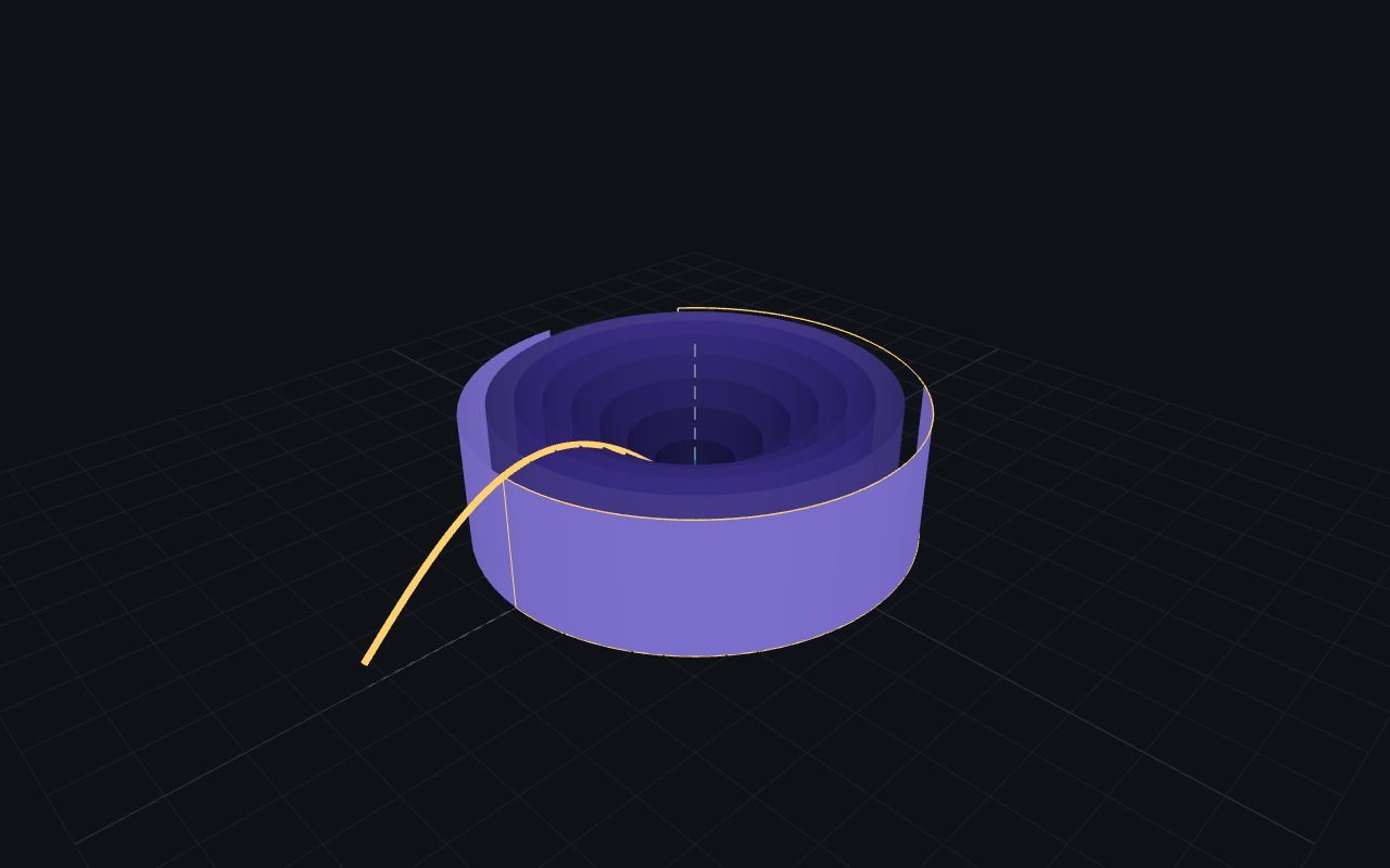
3D rendering of nested cylindrical shells

Shell method.

V = ∫ 2π · x · f(x) · dx
Open
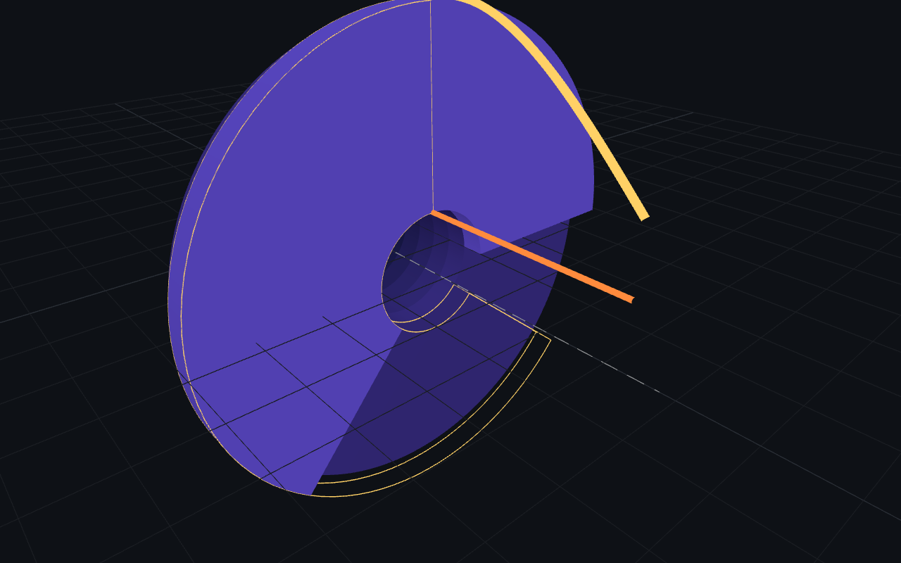
3D rendering of stacked annular washers

Washer method.

V = π ∫ (f(x)² − g(x)²) · dx
Open
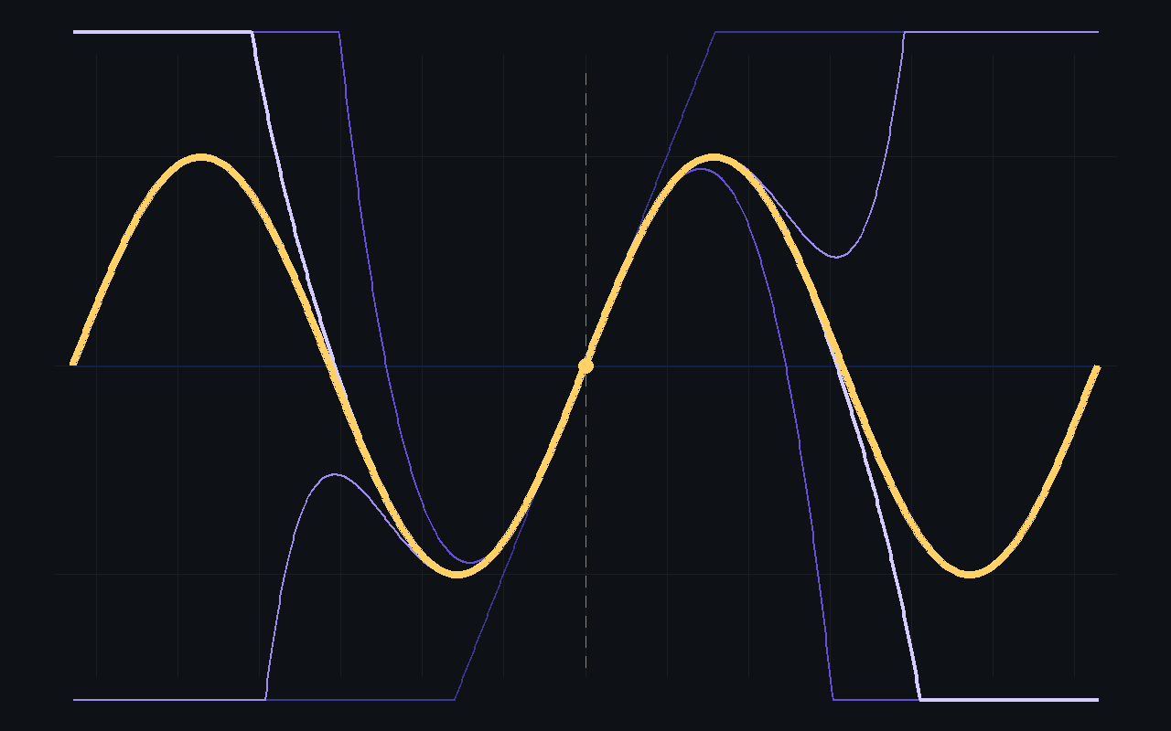
Polynomial approximations converging on a sine curve

Taylor series.

f(x) ≈ Σ fⁿ(a)/n! · (x−a)ⁿ
Open

End behavior.

limx→∞ f(x) = ?
Open

Riemann sums.

∫_a^b f(x) dx ≈ Σ f(x_i*) · Δx
Open

Polar area.

A = ½ ∫ (r₁² − r₂²) · dθ
Open

Vectors & fields

See projection, orientation, rotation, flow, and work as spatial relationships.

Dot product.

a · b = |a||b| cos θ
Open

Cross product.

|a × b| = |a||b| sin θ
Open

Curl. ∇ × F.

curl F = ∂Q/∂x − ∂P/∂y
Open

Divergence. ∇ · F.

div F = ∂P/∂x + ∂Q/∂y
Open

Line integral.

W = ∫_C F · dr
Open

Multivariable calculus

Connect surfaces, level sets, local approximations, and constrained change.

Lagrange multipliers.

∇f = λ ∇g, on g(x,y) = c
Open

Gradient descent.

x ← x − η ∇f(x)
Open

Tangent plane.

z ≈ f(a,b) + f_x · Δx + f_y · Δy
Open

Double integral.

∬_R f(x,y) dA = lim Σ f(x_i,y_j) ΔA
Open

Streamlines. Flow.

dr/dt = F(r)
Open

Contour plots.

f(x, y) = c → level curve
Open

Differential equations

Step through how a local slope rule grows into an approximate solution curve.

Euler's method.

yₙ₊₁ = yₙ + h · f(xₙ, yₙ)
Open